02 - Fastq format sequence files
fastq_files.RmdPreamble
This fastq_processing vignette re-introduces some of the content from the BasicQC tutorial concept but derives the primary information from the FASTQ file for users who have not maintained their sequencing_summary file. This is intended to facilitate the development of workflows and reports that are decoupled from the requirement for the sequencing_summary file.
Getting started with the canned dataset
The floundeR package is distributed with a collection of canned datasets. These include an example FASTQ file that has been gzip compressed and contains a somewhat lacklustre historical dataset that is interesting only in its compactness.
library(floundeR)
#> floundeR v0.0.4

canonical_fastq <- flnDr("example.fastq.gz")
fastq <- Fastq$new(canonical_fastq)
#> → opening fastq stream

print(fastq)
#> <floundeR::Fastq>

fastq$as_tibble()
#> # A tibble: 625 x 3
#>    sequence_length_template mean_qscore_template passes_filtering
#>                       <int>                <dbl> <lgl>
#>  1                      481                 8.58 TRUE
#>  2                      700                 8.94 TRUE
#>  3                      722                 8.71 TRUE
#>  4                      402                 8.68 TRUE
#>  5                      840                 8.77 TRUE
#>  6                      351                 8.55 TRUE
#>  7                      780                 9.18 TRUE
#>  8                      784                 9.07 TRUE
#>  9                      803                 8.67 TRUE
#> 10                      769                 8.46 TRUE
#> # … with 615 more rows
So what have we done here? We have identified the packaged fastq file and we have used this file to instantiate the Fastq object - this can be displayed using the print() command and we can have a quick look at the data that has been extracted using the $as_tibble() function that is exported by the package.
fastq %>% to_sequencing_set()
#> <floundeR::SequencingSet>
The SequencingSet in turn has a collection of methods that can be used to structure and visualise the data. The first that we’ll have a look at is the $enumerate method that returns an Angenieux object for data visualisation.
knitr::include_graphics(
  fastq$sequencingset$enumerate$to_file("figure_5.png")$plot())
#> saving plot as [png]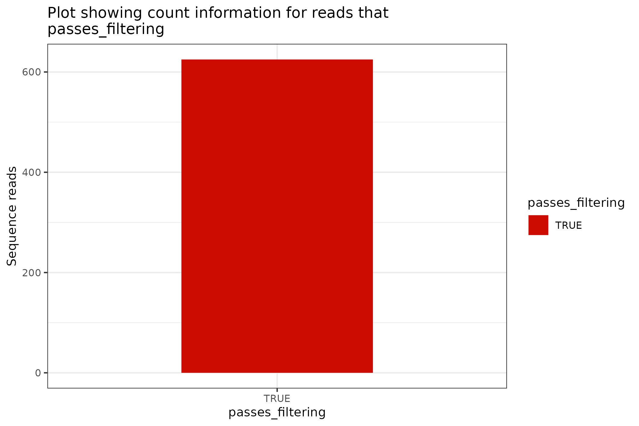
There are a plethora of ways through which the Angenieux object can be used to style, colour and manipulate the graph - please do have a look at the methods documentation.
The SequencingSet object can also be used to access simple but primitive summary statistics such as mean sequence length, N50 length etc
fastq$sequencingset$N50
#> [1] 1156
fastq$sequencingset$mean
#> [1] 1071.438
Review sequence length distributions
The distribution of sequence lengths is an important metric that is impacted by choice of library preparation, starting DNA isolation etc. A plot of length distributions is prepared from the same SequencingSet object that we reviewed in the previous section.
knitr::include_graphics(
  fastq$sequencingset$read_length_bins(bins=35, outliers=0.001)$
    to_file("figure_6.png")$
    plot(style="stacked"))
#> saving plot as [png]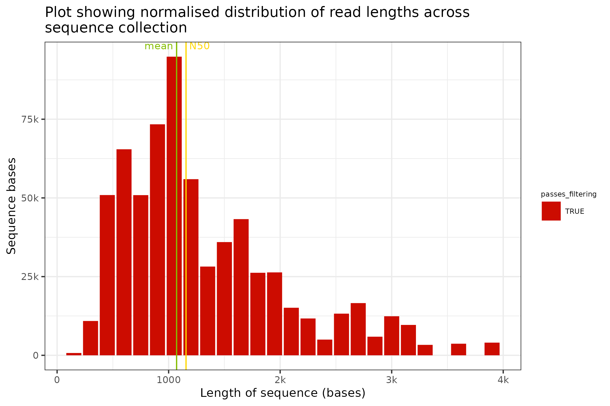
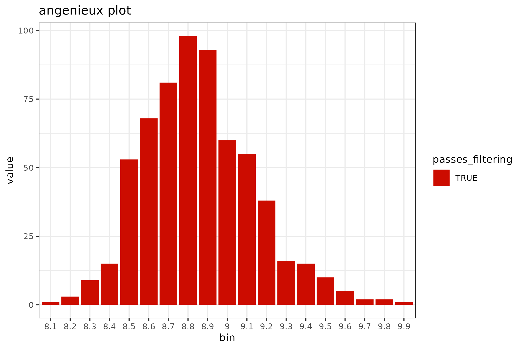
Review quality distributions
The distribution of sequence lengths is an important metric that is impacted by choice of library preparation, starting DNA isolation etc. A plot of length distributions is prepared from the same SequencingSet object that we reviewed in the previous section.
knitr::include_graphics(
  fastq$sequencingset$quality_bins(bins=100)$
    to_file("figure_7.png")$
    plot(style="stacked"))
#> saving plot as [png]